

In this article, I explore several time-series datasets to train a variety of linear models to predict prices of ammunition. I demonstrate how accounting for past world events can reduce prediction error, especially around COVID, and how combining additional regressors can help model performance such as those found in commodities markets. The code used to do the analysis can be found here.
If you have ever taken up competitive shooting like USPSA, IDPA, or PCSL, you will realize that ammunition costs can quickly get expensive as you participate in more matches. For example: if you participate in one USPSA pistol match every weekend, you are very likely to go through about 800 rounds a month, on top of all the ammunition needed for practice. For instance: Ben Stoeger, a well-known USPSA competitor, has mentioned he can go through as much as 550 rounds in a single 80-minute practice session! At the time of this writing, just going to a USPSA match every weekend can be as much as $200 a month in ammunition. If you participate in multi-gun matches, the cost can easily double or triple.
Furthermore, ammo prices are relatively unstable. For example: between mid-2020 and the end of 2021, the industry came under a quadruple whammy when a pandemic, import restrictions, riots, and an election caused prices of .223 Remington to triple (at its peak). In comparison, a gallon of gasoline rose about 70% in the same time period and milk rose about 30%. As you can see, there is some demand for arbitrage in buying ammo, not so much to resell it, but to lessen the financial pain of an already expensive hobby. Thus, having some way to model future prices can be useful. In this study, I chose to build a supervised learner trained on past ammunition data to help predict future prices.
The ammo pricing data I chose to use came from Southern Defense. Depending on the caliber you choose, you can generally find daily and hourly pricing from today all the way back to June 7th, 2020. For this study, I'm using daily data from June 7th, 2020, to August 6th, 2024 (i.e. 1522 days). It is important to note that the actual cost of ammo is going to be higher than the “price” in this database for the following reasons:
In my experience, you generally need to add 30-50% to these prices to get a more realistic cost that includes shipping from more trustworthy sellers. Nonetheless, this is probably the longest running public data source for ammo pricing.
I decide to pick three calibers to analyze: 9x19 mm, .223 Remington, and 7.62x39 mm. I chose these three not only because they are very popular in recreational shooting, but also because they represent different characteristics in the market: 9x19 mm is an extremely ubiquitous pistol cartridge that is popular in competitions, law enforcement, and those interested in self-defense while having a myriad of different loadings from many manufactures..223 Remington, substituting for 5.56x45 mm due to having more data and being virtually interchangeable, is interesting since much of the manufacturing can get tied up in military contracts or government facilities. World events or domestic policy might influence prices more since 5.56x45 mm is the intermediate cartridge for NATO. This contrasts with 7.62x39 mm, while still popular (although less so in the US), has considerably less manufactures with almost all imports coming from a few large, often state-sponsored, factories from overseas. Since 7.62x39 mm is mostly imported, it is sensitive to US foreign policy such as tariffs or bans via executive order.
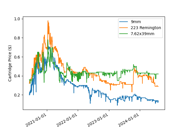
Figure 1 is a plot of raw cartridge price vs. time for the past three years. When first looking at this data, it's clear that the Covid era caused a price spike, although it's difficult to discern much else due how noisy the day-to-day changes are.
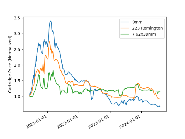
To get a better comparison, I normalized each dataset by dividing by their initial prices (so they all start at "1") to get an idea of growth relative to each-other (Figure 2). I also applied an exponential moving average to smooth out the noise. The results are much clearer: 9mm had the biggest price swing, rising almost 3.5x then crashing to 50% of the original price. 7.62x39 mm rose less than 2x then quickly returned to the starting price and stayed close to there. .223 was somewhere in between.
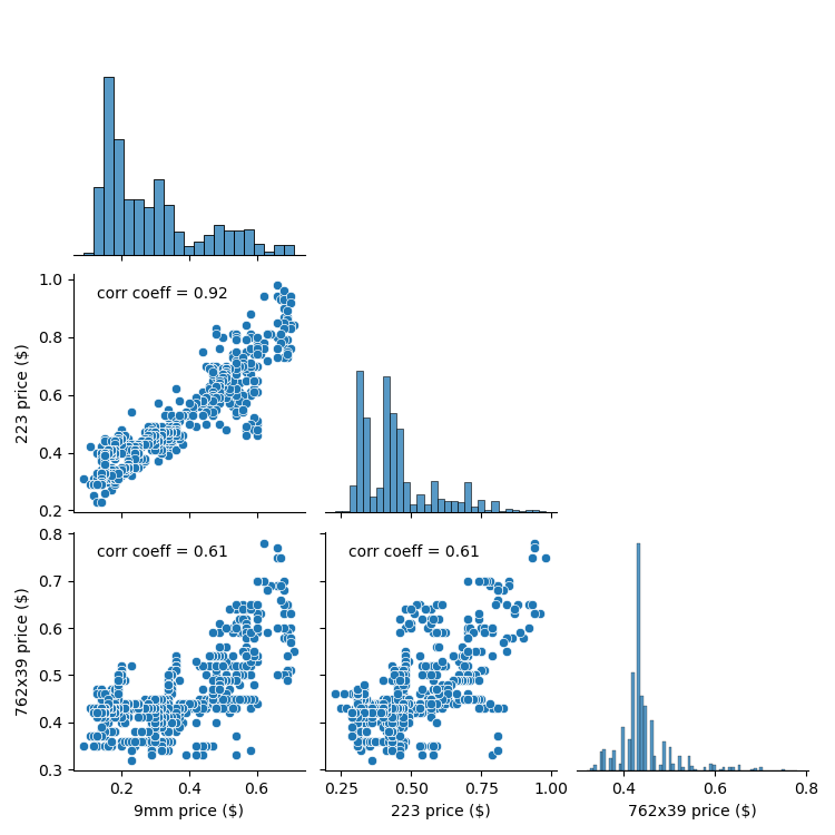
Prices also seem to track each other since the beginning of the dataset and can be seen more clearly in pair-wise scatter plots as shown in Figure 3. We can see some linear correlation between the prices: their correlation coefficients range from 0.61 to 0.92 where 7.62x39mm had tracked each caliber the weakest.
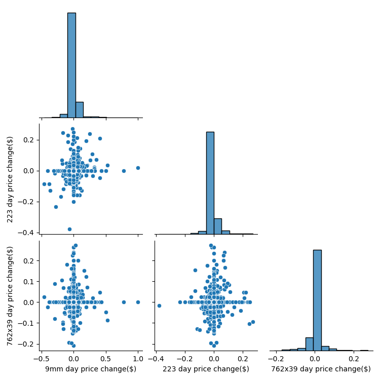
However, when tracking daily price changes, they have almost no correlation with each other. This means that while prices might be indicators of each-other over years, they don't have a fine enough resolution to track day-to-day.
To perform further analysis and regression on the time series data, I decided to try Facebook Prophet as it can supposedly plot trends, seasonality, and model data very quickly and easily. Prophet relies on a linear model which might risk under-fitting the data, but I figured it should provide a good baseline especially considering the relatively small amount of data. The equation representing Prophet's forecasting model as described in the Forecasting at Scale paper looks as follows:
y(t) = g(t) + s(t) + h(t) + eps.
Where y(t) is the price at a certain time step t, g(t) is the trend function (long-term changes/growth that usually looks like a piecewise function), s(t) being the periodic changes (like yearly seasonality effects and tend to look sinusoidal), h(t) being value change due to holiday effects (influence on specific days which tend to just look like step functions), and eps being the error which is otherwise not captured by the model.
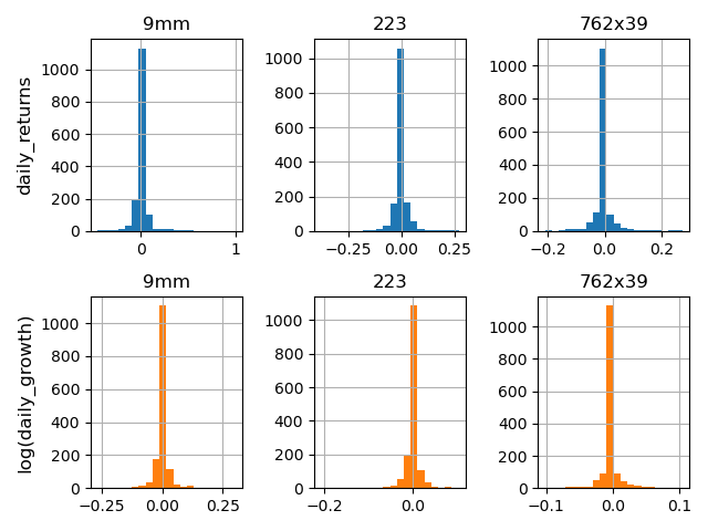
To check if any of the caliber models should be additive or multiplicative (i.e. variance of price swings depend on current values), I did a check described here where one compares histograms of daily returns against the histograms of log(price_i+1/price_i): if the daily return histograms appear more normal, then additive would be more appropriate. From what I could tell, there was little difference between the two sets of plots, so I chose to stick with additive.
From Figure 5, we can see that the largest price swings happened when prices were also high, which might indicate a multiplicative relationship is more appropriate, but these swings also happened around the COVID era. I will later explore ways to handle these swings such as considering holidays and using additional variables.
To start, I chose to model with Prophet's default settings first to get an idea of the trend and seasonality behind each dataset. As seen in the component plots in Figure 6 below (g(t), various s(t)'s), there was clearly an overall spike in trend in beginning of 2021, then a gradual decline since 2022 - this is in line with the raw price plots above (Figure 1).
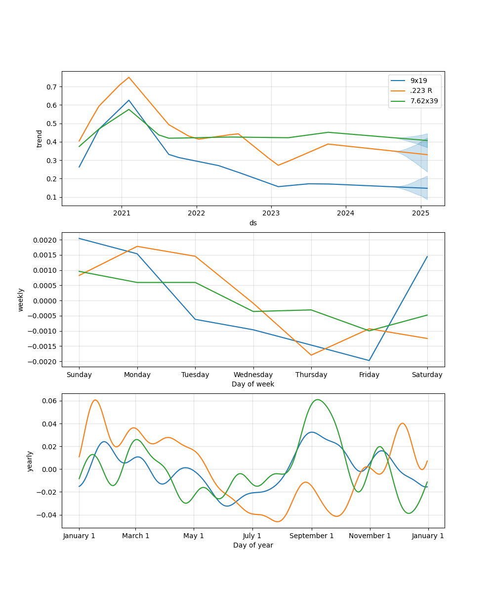
As for weekly seasonality, prices for all calibers seem to reach a minimum around Thursday and Friday, however these changes are within a fraction of a cent and can probably be ignored. The yearly seasonality is much more interesting as there seems to be some non-trivial difference between the calibers. For example, prices seem to peak in September for 9mm and 7.62x39 (coincidentally around Labor Day) while they are almost at a minimum for .223 R, especially around August and October. Conversely, Prices for .223 R peaks in late January and the beginning of December while 7.62x39 reaches its minimum in the beginning of December followed closely in late April (9mm bottoms out in June). The overall yearly price swings for 9mm are around six cents a round while the rifle cartridges are about 10 cents around: thus, it's probably wise to pick one or two times a year to buy, given there aren't any price spikes on the horizon.
To get an understanding of how well these models were performing, Prophet has a built-in cross validation system where you can specify an initial training period for a model, a time horizon to predict up to, and a stagger period of when to train each model. This trains a set of models to check their predictions with the actual data to calculate multiple errors for each day in the dataset. For this study, I chose to train each model on 730 days (about two years), have them predict up to 180 days into the future, and build one of these models every 90 days. Since I had 1522 days of data, this meant Prophet would build seven models to cross validate for each time-series dataset (basically seven errors to average for each day). I chose to use mean absolute percentage error (MAPE) because the error metric to better compare models of different calibers with each-other – the equation can be seen below:
MAPE = 100 * sum_t( ( A_t – F_t ) / A_t ).
Where At is the actual price a specific day (t) and Ft is the forecasted value. The average MAPE for each day in a prediction horizon for each caliber is shown below.
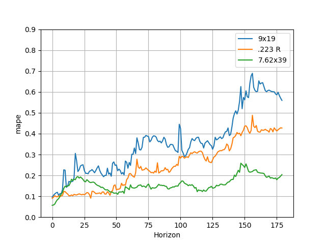
For some reason, it seems that every model has distinct regions of accuracy. For the first two months of prediction, the error of the 9mm and 223 models are relatively minimal, then grow in error further in the future. This makes sense as forecasts should become more unreliable the further into the future as you rely more on extrapolation with old information. 7.62x39 on the other hand seems to spike in error in the first couple months, then calm down afterwards with a constant slight trend upward. My best guess for this is that 7.62x39 pricing is relatively stable over the long term, while short term movements are very noisy. Perhaps 7.62x39 buyers are relatively saturated and newcomers aren't common or popular in times of panic. Regardless, I decided it would be important to monitor the error in these two regions separately moving forward since they behave differently and could reveal certain models performing better in short term or long-term predictions.
Prophet has 15 parameters you can change for a given model. These parameters are easy to tune given the built-in cross validation to check the aggregate performance of each change. The authors of Prophet recommend tuning four of the parameters as per here:
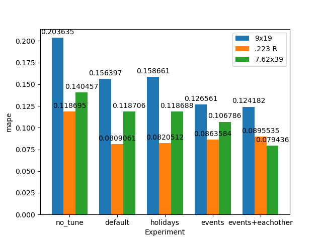
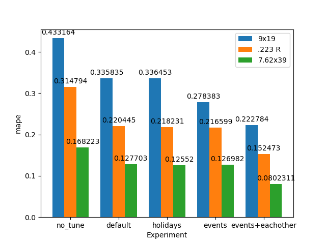
Since I already determined seasonality choice shouldn't matter very much earlier, I chose to ignore it for this study (it would double the grid search space). Since I hadn't incorporated any sort of holidays, I decided to first do a grid search of 16 combinations of the first two parameters to see how the results compared with a default model without any tuning. The results were a 2-4% reduction in average MAPE for the first 60 days of prediction, while reducing error by 4-10% for 60-180 day forecast (the results can be seen in Figure 13). The parameter most responsible for reducing error was lowering seasonality prior scale of the model to its minimum (0.01) while simultaneously increasing changepoint prior scale slightly (from 0.1 to 0.5 depending on the caliber).
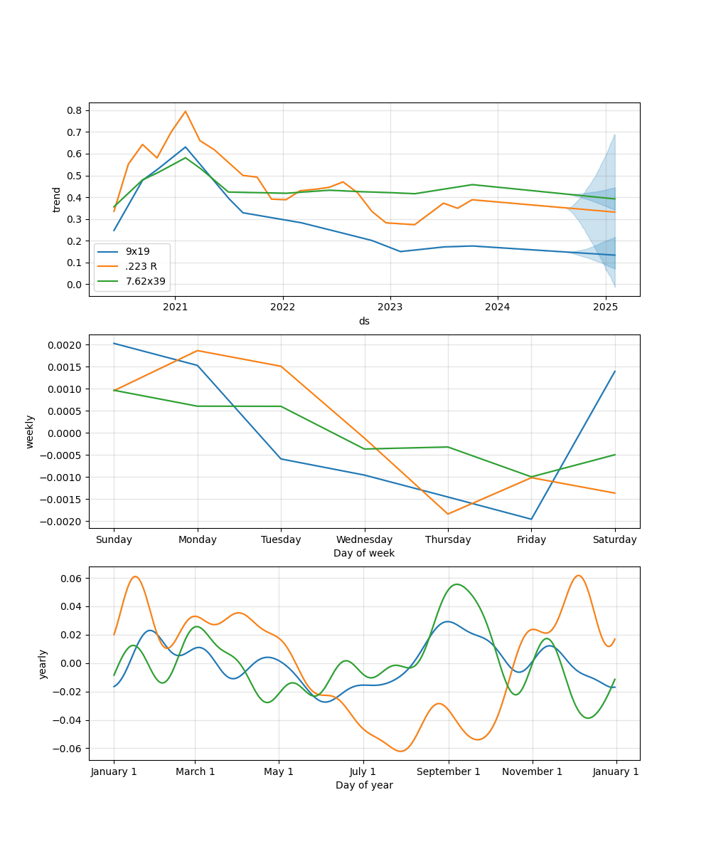
When viewing the new component plots (Figure 8), we can see results in the trend hug the raw data a little more closely especially for 223, although this could be a sign of over-fitting. The seasonality components are basically unchanged. Even though error goes down, the model's forecasting still doesn't really capture the high variance swings in prices especially around the Covid era as seen below in Figure 9. To better capture these, I decided to try to utilize Prophet's "holidays" feature.
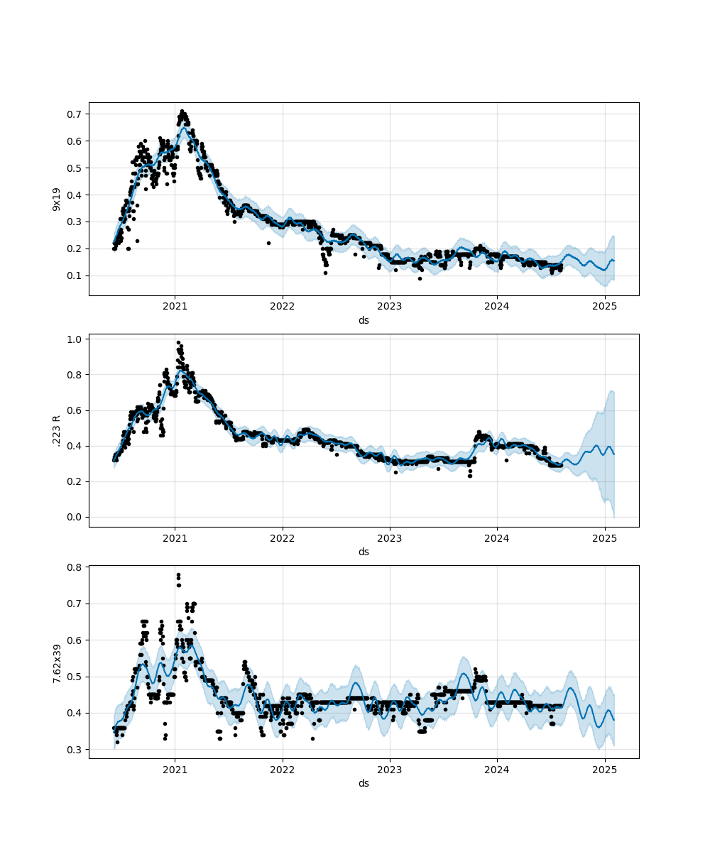
Before trying to model events, I wanted to see if regular recurring US holidays influenced pricing since they typically are associated with sales. Thankfully this is simple in Prophet by just using the "add_country_holidays()" method after initializing a model. However, there was almost no effect on model performance as can be seen on Figure 13 despite doing a small grid search of 4 values of "holidays_prior_scale" ranging from 0.01 to 10. My takeaway from this is that holiday sales, in general, probably have little impact on cartridge prices and can probably be ignored when planning when to buy.
Prophet also can use one-time non-recurring holidays. While this can't always help with future prediction, it can help account for anomalies in past data. I decided to use the Prophet manual's suggestion of Covid lockdown dates as well as add some other dates including the start of the Russo-Ukraine war, the invasions in Israel/Lebanon, the ban on Russian imports in 2021, as well as the 2020/2024 elections as seen below:
special_days = pd.DataFrame([
            {'holiday': 'lockdown_1', 'ds': '2020-03-21', 'lower_window': 0, 'ds_upper': '2020-06-06'},
            {'holiday': 'lockdown_2', 'ds': '2020-07-09', 'lower_window': 0, 'ds_upper': '2020-10-27'},
            {'holiday': '2020_elctn', 'ds': '2020-11-03', 'lower_window': 0, 'ds_upper': '2020-11-03'},
            {'holiday': 'lockdown_3', 'ds': '2021-02-13', 'lower_window': 0, 'ds_upper': '2021-02-17'},
            {'holiday': 'lockdown_4', 'ds': '2021-05-28', 'lower_window': 0, 'ds_upper': '2021-06-10'},
            {'holiday': 'import_ban', 'ds': '2021-08-20', 'lower_window': 0, 'ds_upper': '2021-09-07'},
            {'holiday': 'Rs/Ukr war', 'ds': '2022-02-24', 'lower_window': 0, 'ds_upper': '2022-02-24'},
            {'holiday': 'Israel Inv', 'ds': '2023-10-07', 'lower_window': 0, 'ds_upper': '2023-10-27'},
            {'holiday': '2024_elctn', 'ds': '2024-11-05', 'lower_window': 0, 'ds_upper': '2024-11-05'}
        ])
When viewing the forecast plot (Figure 10) utilizing these holidays, you can see the model captures many more of the outlier spikes/drops, but not all of them (as I probably missed a few key events). Regardless, accounting for these holidays helped the model's performance quite a bit despite almost all the holidays being part of the initial two years of training data during cross validation and not part of the prediction. It should be mentioned that the same grid search for holiday prior scale was as used for tuning as described in the US holidays model above.
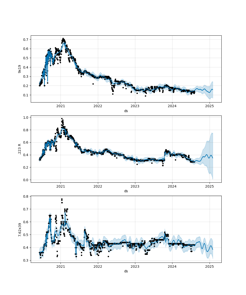
Surprisingly, the rifle cartridge models benefitted the least from these events (.223 R even degraded by ~0.05% in the 60-day forecast) which goes against my hypothesis that wars or bans might affect the ability to predict their prices in general. However, the price spike in .223 R around the invasions in Israel/Lebanon was now captured by the model (this is important as it took nearly a year to recover!). So perhaps using events slightly degrades day-to-day prediction in some cases but can also help account for sudden shocks in markets.
Since I found earlier that cartridge prices track each-other well, I wanted to see how using them as additional regressors to each model would help performance. Since accounting for world events already improved performance, I left it in as well. With added regressors, the 0–60-day average MAPE decreased about 0.2-3% (although degraded .223 R by about 0.02%), and all models improved by 4.5-6% in the 60–180-day forecast. If you look at the raw MAPE plot, this has the effect of basically flattening out error over the long term as errors are almost entirely under 30% for all calibers even up 180 days.
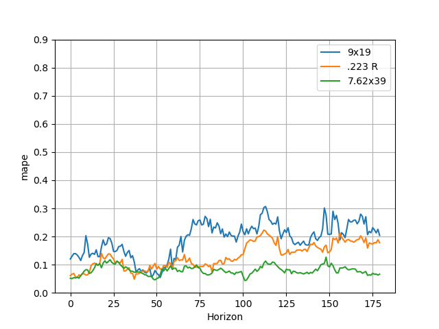
Interestingly, almost all calibers price predictions perform their best between 30 and 60 days with all errors being under ~10%. My guess for this is that price data is quite noisy in the short term as seen in the earlier daily-return scatter plots (Figure 4). Upon viewing the forecasts for each model across the entire dataset, it can be seen the model starts to capture more of the outlier events which might mean certain calibers can be used as leading indicators. Example: perhaps if one caliber is becoming expensive, it causes people to start buying another later. This change also tightened the 80% confidence bound around the predictions in the improved model, especially for the 223.
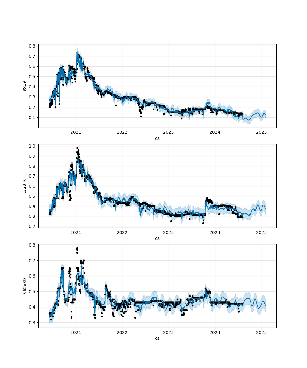
To better visualize how each method performs against each-other, I took the average of the 0-60 day and 60-180 day forecast MAPEs and plotted them below (Figure 13).
Since using other cartridge prices seemed to help predict prices better, I wanted to explore other sources of data to see if I could further improve performance. These included:
CCI is an arbitrary score of consumer spending and saving surveys with the scale being set to being "100" over the long-term average (higher is more confident). My thought is that less confident consumers might buy less ammunition when times are tough. It should be mentioned that CCI for a given month is published at the last Tuesday, so scores published by OECD as being the first of every month is a retro-active labeling (nobody knows the score that early). To account for this, I offset each score by the day they are published to prevent the model from "looking ahead.”
Copper is used both in bullet jackets as well as brass, so it seemed like a logical choice to use copper futures to help predict cartridge prices. The primary ingredient in smokeless gunpowder, the propellant of most modern cartridges, is nitrocellulose which is mostly made of cellulose: the most popular source of that being cotton. To account for energy to both produce and transport ammunition (and maybe to make some of the synthetic ingredients in smokeless powder), I also included crude oil and natural gas prices as well. All prices were from day closing.
When viewing the raw scatter plots of each-other's prices (for the same 1522 days as the ammunition price data), the correlations are quite strange, as shown in Figure 14 below:
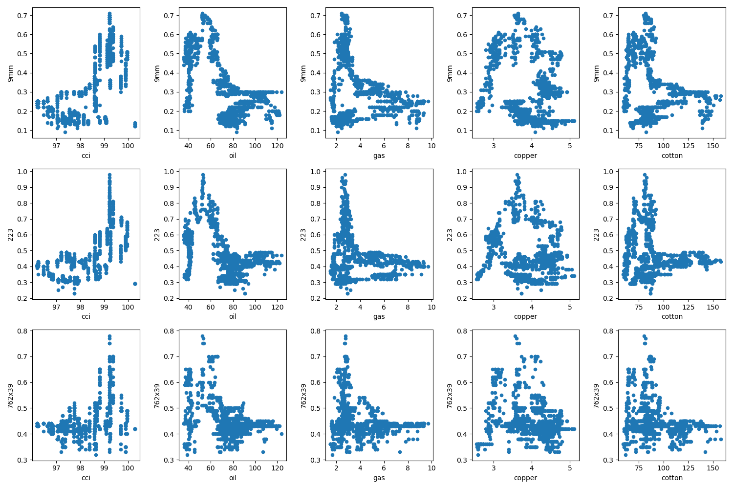
Outside of CCI, which might have a loose exponential relationship, the correlations were almost "L" shaped. At first, one would think this means low commodity prices cause a spike in cartridge prices, but there are many spots where cartridge prices are also low in these regions: the only exception being crude oil in which prices clearly jump below $70 a barrel. Thus, I didn't have much hope Prophet's linear modeling could do much with the data without some sort of transformation.
For this portion of the study, I initially ignored using event-based holidays to see if these other factors could be used as a substitute. However, I found there be very little improvement over the prior caliber-regressor model with holidays. Using CCI, I was able to reduce 7.62x39 mm prediction error around 1% in the 0-60 and 60-180-day forecasts but provided little to no benefit with the other calibers which are more difficult to predict. My guess for this is that CCI is a lagging indicator as real consumer confidence lags the published score by nearly a month. Since oil had a very distinct but non-linear relationship, I decided to make a Boolean mask and use that as a factor: all prices below $70 would be a "1" (as this is when ammo prices tended to be high) and everything else would be a 0, then use it as a multiplicative regressor. This basically did nothing to help the 60–180-day prediction but did reduce 9mm and 7.62x39 mm 0–60-day errors by 0.5-1.5%. To me, this meant that oil prices could be used as an aid to short-term forecasts, possibly because they help price-in shipping costs which could be important for cheap import ammunition.
Taking this further, I tried mixing up the models by including events. I also made a mixed model that utilized Boolean masked oil prices, events, and cartridge prices together. As expected, events almost always improved performance and the final mixed model was the most accurate (in general). However, this final mixed model wasn't that much of an improvement over the model without oil data: it reduced error in the 0-60 day forecast by 0.1-0.6% while 60-180 forecasts were improved by 0-1%. The results can be seen below (Figure 15).
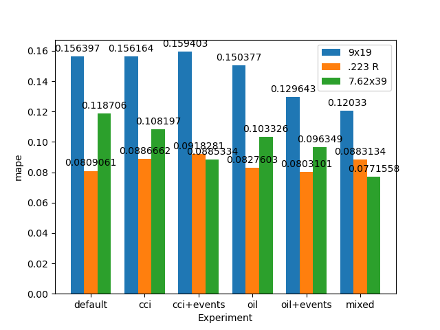
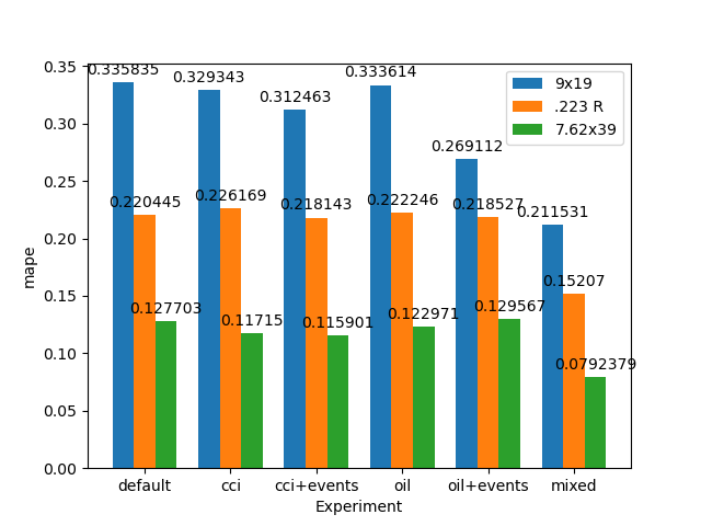
In the end, the best model's average error for the 0–60-day forecast was 12% for 9x19 mm and 7.7% for 7.62x39 mm. If using the combined method of oil and caliber data as additional regressors, .223 R's best error was 8.8%, but was only 8.1% if using just the basic hyper-parameter tuned model with no additional regressors or holidays. For the 60–180-day forecast, the average error was 21% for 9x19 mm, 15% for 223 R, and 7.9% for 7.62x39 mm. The forecasts for this final mixed model method can be seen below (Figure 16):
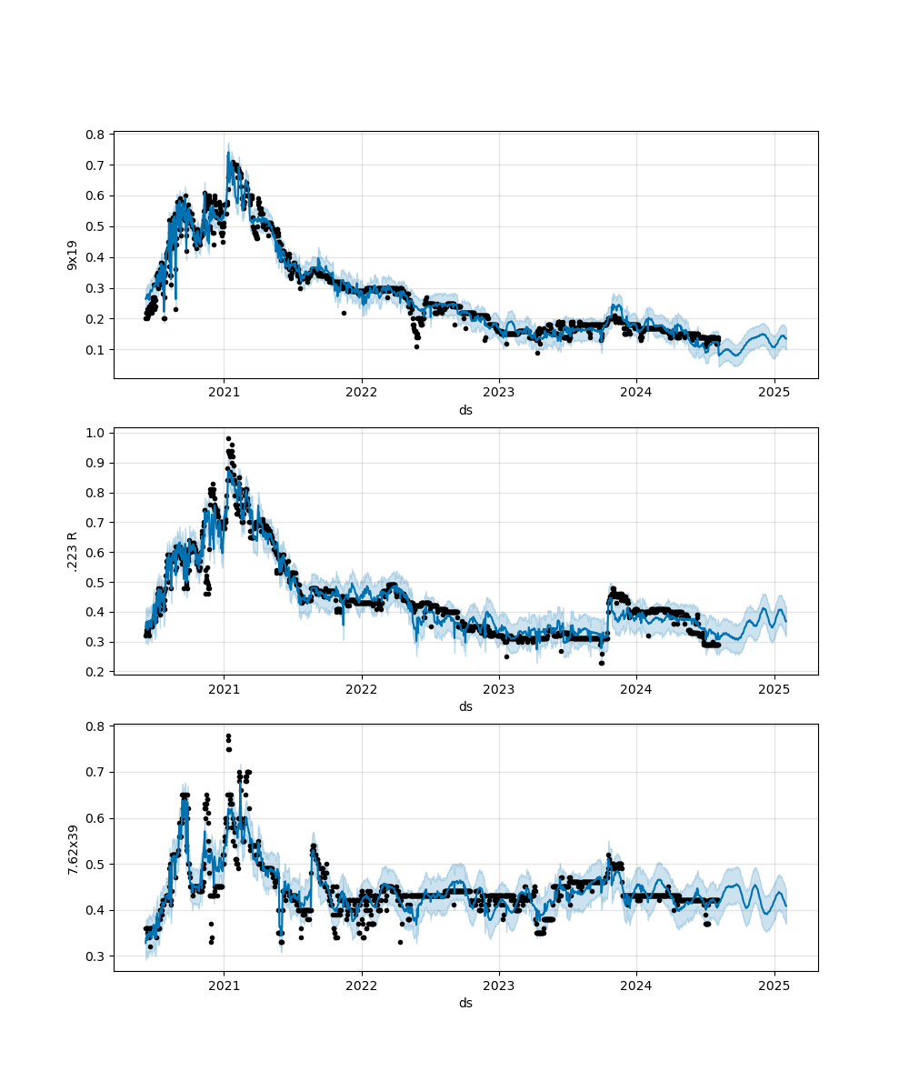
It could be said that this final mixed model followed the actual prices the best with many of the outliers now accounted for. However, 7.62x39's price spikes during COVID are still partially unaccounted for - this sort of makes sense as most of it is imported and I am mostly using US data to try to predict it. Furthermore, much the confidence bound around 7.62x39 mm is still large since Prophet tends to do better with normally distributed historical values than constant ones (the price seems to be very stable past COVID).
I should note that I did try building a model using all futures data as well as CCI (together), but it was harmful to the final performance in almost all instances. This was somewhat expected considering how unusual most of the long-term price relationships where and a linear model probably couldn't make sense of it.
With this Southern Defense dataset, I think using Prophet's default hyper-parameters leaves a lot of improvement of performance on the table and should probably always be tuned before further analysis. Additionally, using world events as holidays and using other calibers as additional regressors helped reduce model error the most. To me, this meant caliber prices, in certain instances, can provide leading indicators to other calibers and should always be incorporated. World events also make past data more useful to help account for anomalous happenings that the model would otherwise attribute to error. While it could be said that other regressors could be helpful, I found that financial data like CCI and commodity futures were too complex for a linear model to use and required manual data transformations that provided little benefit. Oil prices were somewhat helpful, but I am doubtful how they will generalize in the future when most of the ammo price spikes during low oil prices also coincided with the Covid era. It is possible this oil/ammo price relationship will never happen again as it is opposite of intuition.
With all calibers, I would say that the time of year is important when purchasing as there are generally one or two times of the year when it reaches a minimum. It is safe to say that US holidays probably don't affect these prices and that you can also ignore specific days of the week to purchase as well. Otherwise, using forecasts might be most effective to predict one to two months into the future. Pistol ammo prices (9mm) tended to have the highest variance and should be analyzed with shorter term forecasts while longer term forecasts are more reliable for rifle cartridges (223R and 7.62x39).
My overall impression with Prophet is that it is okay for building and tuning a model with one regressor to interpret. However, adding in more regressors is somewhat annoying as you need to build sub-models for each regressor, then manually make predictions with each of them to provide forecast data that an aggregate model can use for prediction. To me, this should be handled by the "make_future_dataframe()" method automatically to prevent a lot of repetitive and error prone busy work. Additionally, the visualization methods require peering into the source code of Prophet to plot multiple models together. Even then, formatting must be done manually afterwards which further builds the case that the library isn't great when utilizing more than one dataset. Lastly, Prophet doesn't have much capacity for sophisticated modeling. Since it is just a linear model, trying to later add in regressors that had non-linear relationships required a fair bit of torturing to try to make them behave linearly. In some cases, this isn't intuitive and can create a lot of grief if you need to switch libraries after finding Prophet isn'tSW powerful enough for your given datasets.
In the future, I would like to incorporate more ammunition data as even two additional regressors tended to help each model tremendously. I also think more sophisticated models might make forecasts more accurate, especially when incorporating data with complex relationships like stock/future data. Perhaps gradient-boosted trees or long-short term memory (LSTM) models could help when stock/future data is included. Lastly, because world events had such a large impact on price prediction, I think having a more programmatic method of determining "happenings" is key to improving performance as we don't always know a day is an "event" until after the fact. Maybe including some sort of sentiment analysis like using X/Twitter posts to help classify days as being "event" holidays would help.